Basics of Machine Learning for Music DSP
Sebastián García Valencia
Note: This web page was done using GitHub pages based on the markdown generated by the python notebook after a complete run to demonstrate the outputs. However, GitHub can’t interpret some things (like the latex formulas) correctly, so just use this page as a preview of the notebook, if you clone the repository and use it in the interactive jupyter environment, all should work.
Requierements
- jupyter==1.0.0
- numpy==1.14.1
- scipy==1.0.0
- scikit-learn==0.19.1
- matplotlib==2.1.2
- librosa==0.6.0
Introduction
The field music DSP is a passionate world where converge many areas like physics, math, engineering, music and computer science. The technics can be used in music information retrieval to make really interesting applications. Besides, the last years we have seen a massive interest in general for machine learning and artificial intelligence, the variety of problems of all conceivable areas that this can resolve is very striking.
The purpose here is showing some of the basics of this two fields, and demonstrate what we can achieve when combining them. At the end of this notebook you will be able of:
- Generate sine waves and export them as wav files
- Transform raw audio to spectrograms and analyze them
- Generate image databases of spectrograms
- Apply a binary classification that recognizes sound and silence
- Apply a multiclass classification for the musical notes
- Export the trained models to reuse them later
Generating sine waves
One of the fundamental concepts in audio (and digital signal processing in general) is the sine wave. When you study the field more in depth, you will know that every signal possible can be modelled as a sum of sine waves with different frequencies, amplitudes and phases. Specifically, these 3 parameters constitute the sine wave formula (which varies over time)
where A is the amplitude, f is the frequency and $\phi$ is the phase
Let’s start defining 2 methods, one to create a signal made of a sine wave of one second and a silence of one second. The other to take a sine wave and export it as a wav sound file.
import numpy as np
import wave
import struct
import matplotlib.pyplot as plt

num_samples = 41100
# The sampling rate of the analog to digital convert
sampling_rate = 41100.0
amplitude = 16000
# creates a sine wave with the given frequence of one seconde and a silence of one second
def make_sound_and_silence(freq=1000):
    # frequency is the number of times a wave repeats a second
    frequency = freq
    sine_wave_part = [np.sin(2 * np.pi * frequency * x/sampling_rate) for x in range(num_samples)] + [0] * num_samples
    return sine_wave_part
nframes=num_samples
comptype="NONE"
compname="not compressed"
nchannels=1
sampwidth=2

# recieves and array with a sine wave and creates a wav file
def save_wav(sine_wave, file = "test.wav"):
    wav_file=wave.open(file, 'w')
    wav_file.setparams((nchannels, sampwidth, int(sampling_rate), nframes, comptype, compname))
    for s in sine_wave:
       wav_file.writeframes(struct.pack('h', int(s*amplitude)))
Let’s generate a sine wave with a frequency of 1000.
little_sine_wave = make_sound_and_silence(1000)

print(little_sine_wave[:10])
print(len(little_sine_wave))

save_wav(little_sine_wave, "shorttest.wav")
print("ready!!!")
[0.0, 0.15228077625453545, 0.30100953426472493, 0.44271710822445204, 0.574098104633321, 0.6920880021007617, 0.7939346326988125, 0.8772623775285732, 0.940127579109596, 0.9810638780730726]
82200
ready!!!
from __future__ import print_function
# We'll need numpy for some mathematical operations
import numpy as np
# matplotlib for displaying the output
import matplotlib.pyplot as plt
import matplotlib.style as ms
ms.use('seaborn-muted')
%matplotlib inline
# and IPython.display for audio output
import IPython.display
# Librosa for audio
import librosa
# And the display module for visualization
import librosa.display
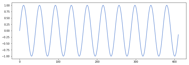
Now let’s listen to the wave and visualize the first millisecond, with a sample rate of 41100 (samples per second) each millisecond will have 411 samples. The frequency of 1000 means, the sine wave makes a complete oscillation 1000 times per second, so in this first millisecond, there should be 10.
# Load the example track
y, sr = librosa.load("shorttest.wav")

# Play it back!
plt.figure(figsize=(12,4))
plt.plot(range(len(little_sine_wave[:411])),little_sine_wave[:411])

IPython.display.Audio(data=y, rate=sr)
[<matplotlib.lines.Line2D at 0x7f5fb92e3690>]
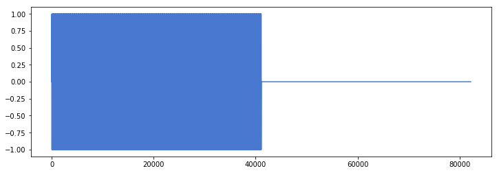
This is the complete wave
plt.figure(figsize=(12,4))
plt.plot(range(len(little_sine_wave)),little_sine_wave)
[<matplotlib.lines.Line2D at 0x7fa4b00cbd10>]
The next step will be generating a signal made of sounds and silences, always with frequencies multiple of 500.
sine_wave=[]
for i in range(1,11):
    sine_wave += make_sound_and_silence(500*i)

print(sine_wave[:10])
print(len(sine_wave))

save_wav(sine_wave, "longtest.wav")
print("ready!!!")
[0.0, 0.07636336493694144, 0.15228077625453545, 0.22730888465333024, 0.30100953426472493, 0.3729523214328617, 0.44271710822445204, 0.5098964759879159, 0.574098104633321, 0.6349470637383889]
822000
ready!!!
y, sr = librosa.load("longtest.wav")
IPython.display.Audio(data=y, rate=sr)
Spectrogram
At this point, it is necessary to speak about another very important concept un DSP. The spectrogram is a way to represent a signal showing the variation of frequency over time. The usual method to generate it is the fast Fourier transform (FFT) which is out of the scope here, but you should read more about it if you want to go more in depth in the topic. The main idea is to have chunks of time and calculate the predominance of some frequencies with the intensity of colours. Said this, can you imagine how should look the spectrogram of “longtest.wav”. In theory, it should be almost black in all the frequencies except the respective multiple of 500, this should change every second, and in the silence parts there should be black vertical rectangles:
# Let's make and display a mel-scaled power (energy-squared) spectrogram
S = librosa.feature.melspectrogram(y, sr=sr, n_mels=128)
# Convert to log scale (dB). We'll use the peak power (max) as reference.
log_S = librosa.power_to_db(S, ref=np.max)
# Make a new figure
plt.figure(figsize=(12,4))
# Display the spectrogram on a mel scale
# sample rate and hop length parameters are used to render the time axis
librosa.display.specshow(log_S, sr=sr, x_axis='time', y_axis='mel')
# Put a descriptive title on the plot
plt.title('mel power spectrogram')
# draw a color bar
plt.colorbar(format='%+02.0f dB')
# Make the figure layout compact
plt.tight_layout()
plt.savefig("testSpectrogram.png")
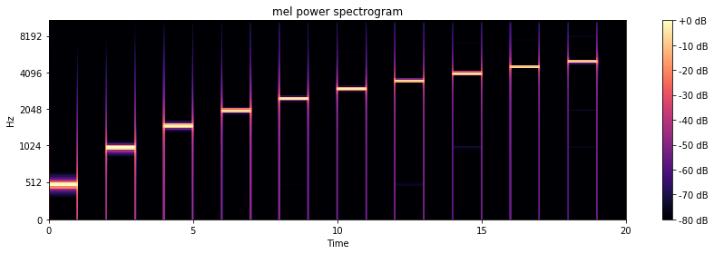
As you can see, this gives a lot of information and being an image, ideas for using it with machine learning come to the mind.
Machine Learning
The basic idea in machine learning is creating models which learn by itself the hidden patterns in the data without having to program it explicitly. There many subdivisions like unsupervised learning (clustering, anomaly detection, etc.) and supervised learning. The second has at the same time a distinction depending on if the data is continuous (regression) or categorical (classification), and the idea is giving labels to the data. I’ll focus on the classification image problem.
create a dataset with each second of a wav
The starting point is to create the data, first, let’s take the spectrogram and delete all the extra information like axis, text, etc
S = librosa.feature.melspectrogram(y, sr=sr, n_mels=128)
log_S = librosa.power_to_db(S, ref=np.max)
plt.figure(figsize=(12,4))
librosa.display.specshow(log_S, sr=sr)
<matplotlib.axes._subplots.AxesSubplot at 0x7fa4aa5ec0d0>
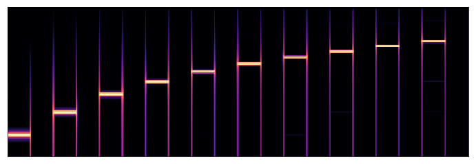
Let’s write a method that creates a dataset folder with a given wav file, making an image of the spectrogram of each second and using the image name as label container (0 for silence and 1 for sound)
# create a dataset with each second of a wav
def create_dataset(audio_path, dataset_name="dataset"):

    y, sr = librosa.load(audio_path)

    #use sr (sampling rate) to split data in seconds
    import os
    if not os.path.exists(dataset_name):
        os.makedirs(dataset_name)

    initial = 0
    final = sr
    for i in range(len(y)/sr):
        # Let's make and display a mel-scaled power (energy-squared) spectrogram
        S = librosa.feature.melspectrogram(y[initial:final], sr=sr, n_mels=128)

        # Convert to log scale (dB). We'll use the peak power (max) as reference.
        log_S = librosa.power_to_db(S, ref=np.max)

        # Make a new figure
        plt.figure(figsize=(12,4))


        # Display the spectrogram on a mel scale
        # sample rate and hop length parameters are used to render the time axis
        librosa.display.specshow(log_S, sr=sr)

        #create dataset with 0 for silence and 1 for sound
        if i % 2 == 0:
            plt.savefig(dataset_name + "/second_"+str(i)+"_label_1.png")
        else:
            plt.savefig(dataset_name + "/second_"+str(i)+"_label_0.png")
        initial += sr
        final += sr
Now, let’s create the dataset
create_dataset("longtest.wav")

print(len(y))
print(sr)
len(y)/sr
441000
22050


20




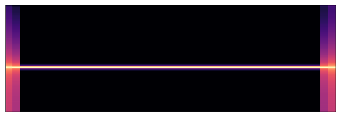

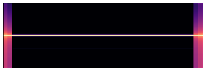

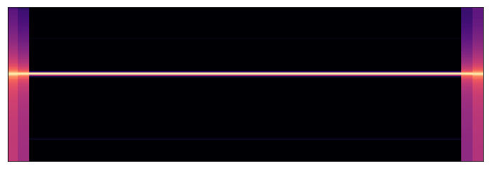

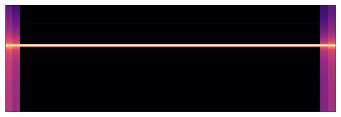

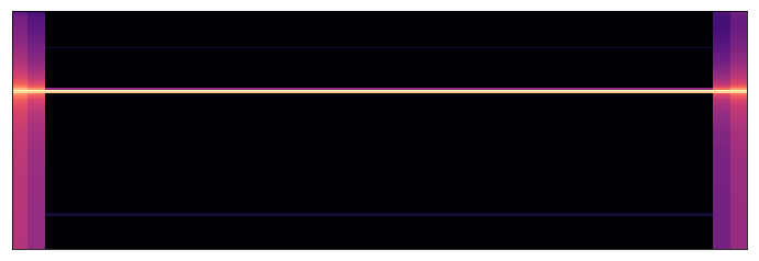

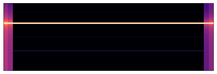

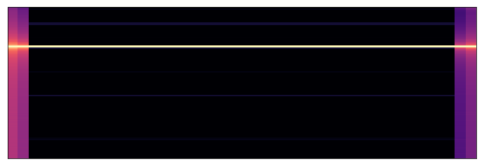

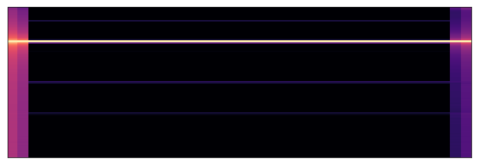

Binary classification
This problem (classificate as silence or sound) is known as binary classfication, I’ll use the simplest calssification model and also, the canonic election for binary classification: logistic regresion
The first step is to prepare the data in the format of flat matrix representations of the images (data), the images itself (images) and the labels obtained from the image file name (labels)
import os
# Standard scientific Python imports
import matplotlib.pyplot as plt

# Import datasets, classifiers and performance metrics
from sklearn import datasets, svm, metrics

def load_data(folder = "dataset"):
    images = []
    labels = []

    for image in os.listdir(folder):
        print(image)
        images.append(plt.imread(folder + "/" + image))
        labels.append(int(image.split("_")[3].split(".")[0]))

    images = np.array(images)
    labels = np.array(labels)
    print(labels)
    images.shape

    # To apply a classifier on this data, we need to flatten the image, to
    # turn the data in a (samples, feature) matrix:
    n_samples = len(images)
    data = images.reshape((n_samples, -1))

    return data, images, labels
data, images, labels = load_data()
second_0_label_1.png
second_15_label_0.png
second_17_label_0.png
second_18_label_1.png
second_16_label_1.png
second_19_label_0.png
second_12_label_1.png
second_6_label_1.png
second_2_label_1.png
second_3_label_0.png
second_1_label_0.png
second_5_label_0.png
second_7_label_0.png
second_13_label_0.png
second_11_label_0.png
second_8_label_1.png
second_4_label_1.png
second_10_label_1.png
second_9_label_0.png
second_14_label_1.png
[1 0 0 1 1 0 1 1 1 0 0 0 0 0 0 1 1 1 0 1]
Logistic Regression
The basic idea is to $\beta_0$ and $\beta_1$ that optimize the logistic function
which has and s form whit a range between 0 and 1 (the labels)
import numpy as np
import matplotlib.pyplot as plt
plt.figure(figsize=(20,4))
from sklearn.model_selection import train_test_split
<matplotlib.figure.Figure at 0x7fa4aa131a90>
The standard procedure is to split the data into train and test data, the first to train the model and the second to measure is performance.
images_and_labels = list(zip(images, labels))
for index, (image, label) in enumerate(images_and_labels[:4]):
    plt.figure(figsize=(12,4))
    plt.subplot(1, 5, index + 1)
    plt.axis('off')
    plt.imshow(image, cmap=plt.cm.gray_r, interpolation='nearest')
    plt.title('Training: %i\n' % label, fontsize = 20)


x_train, x_test, y_train, y_test = train_test_split(data, labels, test_size=0.3, random_state=0)

from sklearn.linear_model import LogisticRegression

# all parameters not specified are set to their defaults
logisticRegr = LogisticRegression()

logisticRegr.fit(x_train, y_train)

predictions = logisticRegr.predict(x_test)
print("Predictions for test:")
print(predictions)

# Use score method to get accuracy of model
score = logisticRegr.score(x_test, y_test)
print("score:")
print(score)
Predictions for test:
[0 0 1 1 0 1]
score:
1.0
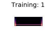
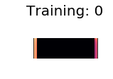

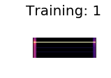
As you can see, the model achieves a score of 100%. This is cause the problem is very simple, so the model can easily memorize all the possible images (overfitting).
Multiclass classification (musical notes)
The challenge now is classifying the 7 fundamental musical notes starting in central C. This kind of problem is known as multiclass classification.
In this case, the procedure changes a little, first let’s define a dictionary with the frequencies of each note (using https://pages.mtu.edu/~suits/notefreqs.html beginning with central C (C4)) and another to map from the note name to the label. Then just create a wav, with random selection of notes from the dictionary, in this case, I’ll use the file name of the wav to store the labels.
notes = {"C" : 261.63, "D" : 293.66, "E" : 329.63, "F" : 349.23, "G" : 392.00, "A" : 440.00, "B" : 493.88}
labels_dict = { "silence" : 0,"C" : 1, "D" : 2, "E" : 3, "F" : 4, "G" : 5, "A" : 6, "B" : 7}
import random

sine_wave=[]
file_name = ""
for i in range(0,20):
    rand_note = random.choice(notes.keys())
    file_name += str(labels_dict[rand_note]) + "_"
    sine_wave += make_sound_and_silence(notes[rand_note])

print(sine_wave[:10])
print(len(sine_wave))

wav_name = file_name + "notes.wav"
save_wav(sine_wave, wav_name)
print("ready!!!")
[0.0, 0.07543046515047773, 0.15043113720275844, 0.22457467196449352, 0.2974386091014805, 0.3686077792623642, 0.43767666966025487, 0.5042517346324829, 0.5679536380132163, 0.6284194145421929]
1644000
ready!!!
Now, to create the dataset I’ll trust in the order of the notes in the file name which corresponds to the order in wav.
# create a dataset with each second of a wav
def create_dataset_notes(audio_path, dataset_name="notesdataset"):

    y, sr = librosa.load(audio_path)

    labels = audio_path.split("_")

    #use sr (sampling rate) to split data in seconds
    import os
    if not os.path.exists(dataset_name):
        os.makedirs(dataset_name)

    initial = 0
    final = sr
    for i in range(len(y)/sr):
        # Let's make and display a mel-scaled power (energy-squared) spectrogram
        S = librosa.feature.melspectrogram(y[initial:final], sr=sr, n_mels=128)

        # Convert to log scale (dB). We'll use the peak power (max) as reference.
        log_S = librosa.power_to_db(S, ref=np.max)

        # Make a new figure
        plt.figure(figsize=(12,4))


        # Display the spectrogram on a mel scale
        # sample rate and hop length parameters are used to render the time axis
        librosa.display.specshow(log_S, sr=sr)

        #create dataset with 0 for silence and 1 for sound
        if i % 2 == 0:
            plt.savefig(dataset_name + "/second_"+str(i)+"_label_" + labels[i/2] + ".png")
        else:
            # we only want the notes in this case
            print("silence")
            #plt.savefig(dataset_name + "/second_"+str(i)+"_label_0.png")
        initial += sr
        final += sr
create_dataset_notes(wav_name, "datasetnotes")
silence
silence
silence
silence
silence
silence
silence
silence
silence
silence
silence
silence
silence
silence
silence
silence
silence
silence
silence
silence


















data, images, labels = load_data("datasetnotes")
second_6_label_7.png
second_18_label_6.png
second_0_label_7.png
second_16_label_1.png
second_36_label_4.png
second_26_label_6.png
second_10_label_7.png
second_14_label_6.png
second_12_label_3.png
second_34_label_5.png
second_20_label_6.png
second_28_label_5.png
second_32_label_3.png
second_38_label_7.png
second_4_label_5.png
second_8_label_1.png
second_24_label_3.png
second_30_label_1.png
second_2_label_2.png
second_22_label_4.png
[7 6 7 1 4 6 7 6 3 5 6 5 3 7 5 1 3 1 2 4]
Support Vector Machine (SVM)
With random forest and neural networks, support vector machines are one of the most potent methods for classification. The basic idea of SVM is to generate hyperplanes in multidimensional spaces which separates the different categories into groups.
images_and_labels = list(zip(images, labels))
for index, (image, label) in enumerate(images_and_labels[:4]):
    plt.subplot(2, 4, index + 1)
    plt.axis('off')
    plt.imshow(image, cmap=plt.cm.gray_r, interpolation='nearest')
    plt.title('Training: %i' % label)

n_samples = len(images)

# Create a classifier: a support vector classifier
classifierSVM = svm.SVC(gamma=0.001)

# We learn the digits on the first half of the digits
classifierSVM.fit(data[:n_samples // 2], labels[:n_samples // 2])

# Now predict the value of the digit on the second half:
expected = labels[n_samples // 2:]
predicted = classifierSVM.predict(data[n_samples // 2:])

print("Classification report for classifier %s:\n%s\n"
      % (classifierSVM, metrics.classification_report(expected, predicted)))
print("Confusion matrix:\n%s" % metrics.confusion_matrix(expected, predicted))

images_and_predictions = list(zip(images[n_samples // 2:], predicted))
for index, (image, prediction) in enumerate(images_and_predictions[:4]):
    plt.subplot(2, 4, index + 5)
    plt.axis('off')
    plt.imshow(image, cmap=plt.cm.gray_r, interpolation='nearest')
    plt.title('Prediction: %i' % prediction)

plt.show()
Classification report for classifier SVC(C=1.0, cache_size=200, class_weight=None, coef0=0.0,
  decision_function_shape='ovr', degree=3, gamma=0.001, kernel='rbf',
  max_iter=-1, probability=False, random_state=None, shrinking=True,
  tol=0.001, verbose=False):
             precision    recall  f1-score   support

          1       0.67      1.00      0.80         2
          2       0.00      0.00      0.00         1
          3       1.00      1.00      1.00         2
          4       1.00      1.00      1.00         1
          5       1.00      1.00      1.00         2
          6       1.00      1.00      1.00         1
          7       1.00      1.00      1.00         1

avg / total       0.83      0.90      0.86        10


Confusion matrix:
[[2 0 0 0 0 0 0]
 [1 0 0 0 0 0 0]
 [0 0 2 0 0 0 0]
 [0 0 0 1 0 0 0]
 [0 0 0 0 2 0 0]
 [0 0 0 0 0 1 0]
 [0 0 0 0 0 0 1]]
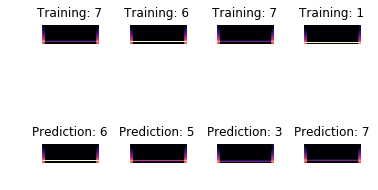
Here are reported 3 different metrics of the model. The intuitive description is: precision tells how much of what the model predicts is correct, recall tells which portion of all that it was possible to predict in the model was correctly predicted, and the f1-score is a combination of both. The confusions matrix relates the true labels with the predicted, to know in which categories the models tend to be “confused”.
Save the train models as pickles
Finally, let’s export the trained models as pickle files, this will be the usual procedure to deploy the model. Later, the model just has to be loaded and used.
import pickle
pickle.dump(logisticRegr, open('logisticRegr.p','wb'))
pickle.dump(classifierSVM, open('classifierSVM.p','wb'))
pretrained_logreg = pickle.load(file('logisticRegr.p'))
print("ready!!!")
ready!!!
pretrained_logreg.predict(data)
array([1, 1, 1, 1, 1, 1, 1, 1, 1, 1, 1, 1, 1, 1, 1, 1, 1, 1, 1, 1])
pretrained_svm = pickle.load(file('classifierSVM.p'))
print("ready!!!")
ready!!!
pretrained_svm.predict(data)
array([7, 6, 7, 1, 4, 6, 7, 6, 3, 5, 6, 5, 3, 7, 5, 1, 3, 1, 1, 4])
Some sources
- https://github.com/librosa/librosa
- https://magenta.tensorflow.org/onsets-frames
- http://pythonforengineers.com/audio-and-digital-signal-processingdsp-in-python/
- https://en.wikipedia.org/wiki/Sine_wave
- https://towardsdatascience.com/logistic-regression-using-python-sklearn-numpy-mnist-handwriting-recognition-matplotlib-a6b31e2b166a
- https://pages.mtu.edu/~suits/notefreqs.html
- http://scikit-learn.org/stable/auto_examples/classification/plot_digits_classification.html